Job Talle

On AI, Art & Algorithms

Simulating hydraulic erosion

Simulating hydraulic erosion

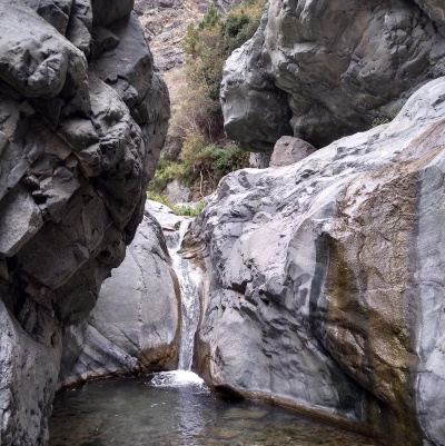
Hydraulic erosion is the process by which water transforms terrain over time. This is mostly caused by rainfall, but also by ocean waves hitting the shore and the flow of rivers. Figure 1 shows the considerable effects that a small stream has had on the rocky environment around it. When creating realistically looking environments, the effects of erosion need to be accounted for. I have experimented with procedural terrain generation before to generate scenes for layered voxel rendering and to demonstrate cubic noise. These terrains were very basic and did not account for erosion. Therefore, they lack a lot of detail, making them unrealistic at closer inspection.

In this article, I will detail a simple and fast method that approximates the effects of hydraulic erosion. The aim of this method is to create believable environments rather than reaching a high degree of realism. Fidelity may be sacrificed for the sake of speed, as long as the results look natural. Summarized, the method should do the following:

• The results must look natural.
• The algorithm must be simple.
• The algorithm must be fast.
• The algorithm should simulate hydraulic erosion caused by rainfall and rivers.

Multiple approaches

There are several different approaches when it comes to simulating erosion. All methods simulate the same phenomenon: water moving from high places to low places, eroding terrain as it flows, and depositing sediment as they go further down their paths. This process always results in a number of recognizable terrain features like gulleys and valleys where rivers flow, deltas where they meet their destination and alluvial fans where smaller streams combine into bigger rivers. While reading about this topic, I have encountered the following distinct strategies in research literature:

• Erosion is simulated by keeping track of where water is for every position on the terrain. A grid (or 2D array) is created for the environment, and water levels and pressures are kept for every cell. When updating, the pressures determine where the water flows to. While flowing, water moves sediment around.
• Erosion is simulated by dropping many particles simulating raindrops on the terrain. The particles then move down the slopes of the terrain. They can bring sediment with them or deposit it.

Mostly for performance reasons, I've chosen to implement a drop based method. Because most drops don't flow very far, many inactive drop simulations can be terminated early and the bulk of the processing power will go to the drops that actually carve out terrain features. The grid based simulation will need to simulate every part on the terrain for every update cycle.

Snowballs

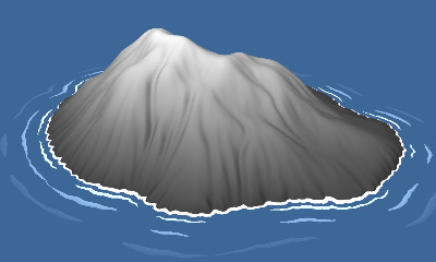
The drops in the simulation can be seen as snowballs instead of raindrops. Within the context of the simulation, I believe this is a better analogy. The snowballs start small when they are dropped, but gain more material as they roll down the hills. When they become too big, they start shedding material as they go. When they stop rolling in valleys or in the sea, the snowballs fall apart and leave their material on the terrain.

The complete erosion algorithm (in Javascript) can be read below. This code uses a heightMap object to erode. This height map can be read from and written to, and the sampleNormal function can be used to get the surface normal. This is a 3D vector pointing upwards from the terrain, so it can be used to determine the slope direction and steepness.

/**
 * Let a snowball erode the height map
 * @param {Number} x The X coordinate to start at
 * @param {Number} y The Y coordinate to start at
 */
trace = function(x, y) {
  const ox = (random.getFloat() * 2 - 1) * radius; // The X offset
  const oy = (random.getFloat() * 2 - 1) * radius; // The Y offset
  let sediment = 0; // The amount of carried sediment
  let xp = x; // The previous X position
  let yp = y; // The previous Y position
  let vx = 0; // The horizontal velocity
  let vy = 0; // The vertical velocity

  for (let i = 0; i < maxIterations; ++i) {
// Get the surface normal of the terrain at the current location
const surfaceNormal = heightMap.sampleNormal(x + ox, y + oy);

// If the terrain is flat, stop simulating, the snowball cannot roll any further
if (surfaceNormal.y === 1)
  break;

// Calculate the deposition and erosion rate
const deposit = sediment * depositionRate * surfaceNormal.y;
const erosion = erosionRate * (1 - surfaceNormal.y) * Math.min(1, i * iterationScale);

// Change the sediment on the place this snowball came from
heightMap.change(xp, yp, deposit - erosion);
sediment += erosion - deposit;

vx = friction * vx + surfaceNormal.x * speed;
vy = friction * vy + surfaceNormal.z * speed;
xp = x;
yp = y;
x += vx;
y += vy;
  }
};

// Simulate 50000 snowballs
const snowballs = 50000;

for (let i = 0; i < snowballs; ++i)
  trace(
random.getFloat() * width,
random.getFloat() * height);

// Blur the height map to smooth out the effects
heightMap.blur();

The algorithm has a few notable properties:

• The variables ox and oy encode the offset of a snowball. They are used to read the terrain slope with a certain offset to make the snowball motion a bit rougher, which prevents snowball paths from converging too much.
• When the surface normal points perfectly upwards (when the y value of that normal equals one), the snowball terminates. In practice, this means that snowballs that have reached the edge of the simulated are or the sea floor stop simulating there. Because nothing happens in those areas, simulating erosion would be a waste of processing power.
• When changing the amount of sediment, the snowball edits the height map at its previous position instead of its current position. Erosion and deposition take place behind it to prevent snowballs from digging themselves in.
• After simulating erosion, gaussian blur is applied to the height map. Because the height map in these examples has a low resolution, blur is required to keep the surfaces smooth enough to be visually appealing.

Because the offset is used while eroding, and because the erosion rate is quite high, every traced snowball has a larger influence on the terrain than a smaller node that looks more like a raindrop would. This results in a fast simulation, but it reduces precision.

Results

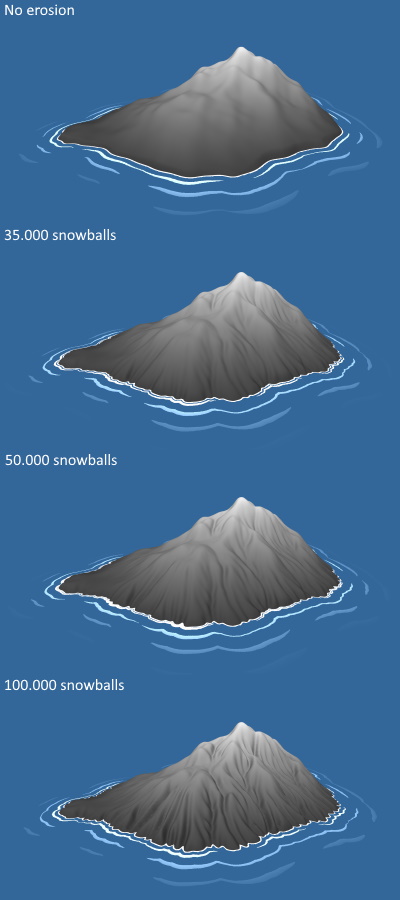
Applying the algorithm above with varying snowball counts gives the results rendered in Figure 3. The algorithm works in a browser, and the source code can be found on GitHub. Pressing the space bar generates a new island. The "starting material" for the algorithm is shown in the first image of figure 3. This island shape was generated using a very similar algorithm to the one I used in my layered voxel rendering example terrains. While the shape does contain some details and ridges, it is very smooth and contains no traces of hydraulic erosion.

The second image shows the same island after dropping 35.000 snowballs on it. They are dropped randomly and evenly spaced. Because of the random initial conditions of the starting shape, valleys and river like structures form where the snowballs find the quickest way to the sea. 35.000 may seem like a high number, but recall that snowballs that reach the sea floor or the edge of the map terminate early. The majority of drops don't fall on the island, so only a small number will actualy roll down one of the valleys that can be seen in the image.

The third image shows the same island after dropping 50.000 snowballs. Compared to the previous image, no new details form, although the terrain features are more pronounced.

The last image shows the island after dropping 100.000 snowballs. This is clearly too much; the ridges become very deep and the shore is very rough. At this point, the results start looking less realistic too. The valleys carve out very sharp terrain features that would erode away themselves.

All islands in the images above can be generated within half a second on my desktop computer, with the algorithm running on a single CPU thread. Therefore, it is not necessary to reduce the number of snowballs for performance reasons in most applications. The algorithm is fast enough as it is.

Conclusion

The proposed algorithm provides a fast method to approximate hydraulic erosion. While realism was no priority, erosion and deposition patterns that one would expect do show up when testing the method on various terrains.

Because the code runs very fast (contrary to most alternative solutions that can be found in the literature), it may be suitable for applications like procedural terrain generation in games. In those applications, it is desirable to produce results quickly, while the results do not need to be very realistic; they just need to look credible.

The method can be extended to track the paths of river beds. Valleys where many snowballs roll through would realistically be rivers. When an area reaches a certain threshold of "snowball traffic", a river or lake can be created there.

Another interesting addition would be a texture that keeps track of the amount of erosion and deposition of material on the terrain. This data can then be used to color the terrain; if lots of material is deposited, sand and small particles will accumulate there. Areas where little erosion has taken place will look different from heavily eroded slopes.

Appendix: rendering shore waves

The animated example contains waves that move towards the shore of the islands. Besides clarifying the shape of the shore, they don't really serve a purpose with regards to the erosion, but it makes the scene prettier.

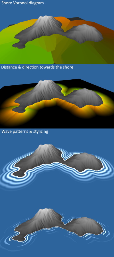
Figure 4 shows the steps that create the wave animation:

1. First, a Voronoi diagram is created around the island shore. Instead of creating a diagram from points, the diagram is created from shapes. Every part of the island that is not under sea level is essentially a point in the Voronoi diagram. This blog post explains the jump flooding algorithm which was used to generate the Voronoi diagram on the GPU; this blog also explains the use of shapes instead of just points when constructing a diagram.
2. After the Voronoi diagram has been created, the data in the diagram is used to create a texture storing the distance and direction to the nearest shore point for every pixel. Figure 4 shows that the red and green channels are used to store the direction vector. The magnitude of that vector encodes the distance to the shore, where the black areas are the furthest away from the shore.
3. A sine wave is created to represent the global wave pattern. The position in the sine wave is determined by the direction towards the nearest shore point, and the wave slowly shifts towards the shore. The direction towards the nearest shore point can be used to calculate the surface normals of the wave shape, if the waves are three dimensional.
4. Finally, the waves are stylized, and the wave patterns are broken up a bit to give the impressions that all waves are their own entities.

This animation shows the steps in figure 4 in real time.