Cubic noise
31 Oct 2017Coherent random noise
Coherent random noise is random noise which is not totally unpredictable; in other words, adjecent values in coherent random noise have some relation to each other, but the noise as a whole is random. An example of pure random noise is white noise, which is produced by a TV if no cable is plugged in. The noise is totally random, no patterns can be recognized. A cloudy sky is an example of coherent random noise. The patterns and shapes of individual clouds cannot be predicted, but the clouds themselves form recognizable features.
Random noise is often used to produce pseudorandom effects in software. A notable example is terrain in games. 2D coherent random noise is produced, and the values are interpreted as a heightmap. An interactive demonstration of this technique can be found further down this page.
Cubic noise
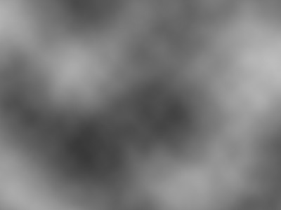
Figure 1 shows an example of cubic noise. Cubic noise is essentially scaled up white noise with cubic interpolation. Cubic interpolation ensures the result is smoothed enough to remove grid like artifacts. The values are based on coordinates, every pixel in this example represents a set of coordinates. These coordinate values can be tiled to make a tiling noise texture. All values produced by the cubic noise algorithm lie within $[0, 1]$.
The cubic interpolation method is as follows:
$$n = x(x(x (-a + b - c + d) + 2a - 2b + c - d) - a + c) + b$$
$a$, $b$, $c$ and $d$ are the four samples to interpolate between, and $x$ is the interpolation position in the range $[0, 1]$, which interpolates the region between $b$ and $c$. The noise value is $n$.
The algorithm for cubic noise can be found in this repository. Implementations for several programming languages are included. The algorithm is very simple, so it can easily be ported to other languages. I have published the repository under the unlicense, so there's no licensing to worry about.
Octaves & falloff
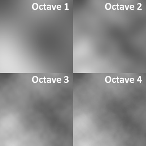
The example in figure 1 shows some small scale detail, instead of just large smooth gradients. This is achieved by adding several octaves to the noise. The first octave has the largest influence and the largest scale (which means it has been zoomed in a lot). Every next octave has smaller influence and a finer scale than its predecessor. This process is shown in figure 2.
Adding octaves presents a challenge. It is important that the sum of all octave influences is one; if this is not the case, the resulting noise will probably be either too dark or oversaturated. I define falloff $f$ as the number each successive octave influence is divided by. For example, if $f = 2$, the initial influence is $\frac{1}{f}$, the next influence is $\frac{\frac{1}{f}}{f}$ and so forth.
The number of octaves is defined as $o$. If $o = 3$, the total influence will be $\frac{1}{2} + \frac{1}{4} + \frac{1}{8} = \frac{7}{8}$. Unfortunately, this does not sum up to one. To normalize the total influence, it needs to be multiplied by the swapped fraction of the total sum (since $\frac{x}{y} * \frac{y}{x} = 1$), which is $\frac{8}{7}$ in this example. I call this normalizer $n$. The influence of the first octave $i$ can now be defined as $i = \frac{n}{f}$, which leads to
$$\sum\limits_{x=1}^{o} \frac{n}{f ^ x} = 1$$
If $n$ can be calculated from falloff and octaves, we have a general formula that yields an initial influence $i$ which will lead to the sum of all octaves being one. Luckily this is possible using the following formula, which calculates the numerator and denominator of the total sum given $f$ and $o$ and swaps them:
$$n = \frac{(f - 1) f ^ o}{f ^ o - 1}$$
$$i = \frac{n}{f}$$
Of course this formula for $i$ will not work when $f = 1$ or $f = 0$ because those values will result in divisions by zero. For $f = 1$, $i = \frac{1}{o}$, since every octave has the same influence. The second case shouldn't occur, because $f = 0$ makes no sense; the influence of every next octave would be infinitely larger than the previous one.
An interactive demonstration of cubic noise with octaves is given below. All previously described parameters can be changed. Every next octave, the period of the noise is halved
| Seed | |
| Quality | |
| Period | |
| Octaves | |
| Falloff |
Applications
Coherent random noise has many applications in pseudorandom number generation. When numbers must be random but not noisy, cubic noise comes in handy. A classic example is random terrain generation. A 2d grayscale noise is generated, and every pixel is translated into terrain height. Additionally, tunnels and caves can be generated by clearing a certain range of values in a 3d noise.
An example of 2D terrain generation is shown below. Terrain is generated from 2d cubic noise. The values on the noise determine terrain height, and the height determines terrain color. By using a height dependent color gradient, water, beaches and snowy peaks can be seen. A power slider is added to add a power to the final value generated by the noise. Height values with a power produce better mountain shapes.
| Gradient style | |
| Seed | |
| Period | |
| Octaves | |
| Falloff | |
| Amplitude | |
| Power | |
| Lower bound |
The example above doesn't do much more than generating a noise with octaves, but the generated terrain already looks decent. There are many ways to improve this. Adding cliffs and irregular terrain features would add some nice variety, and creating continuous rivers would separate different sections of terrain from each other. Erosion could be simulated to make the mountains look much more natural.
A good way to add more variety would be adding biomes. The biome could be determined by sampling a large scale cubic noise, where every biome would be represented by a range of values in the noise. Different biomes can then have different amplitudes, frequencies, features and colors.
Why use cubic noise?
The informed reader may ask, why use cubic noise in particular? The industry standard has been Perlin noise for a while, and to a lesser degree simplex noise. Both algorithms are faster than cubic noise, at least when surrounding values in cubic noise are not buffered. Granted, there are many cases in which Perlin or simplex noise is favorable. Cubic noise however has properties that sometimes come in handy:
- Cubic noise has more variance in its peaks and valleys than perlin noise because of cubic interpolation. If the neighboring tiles have contrasting values, peaks can sometimes be extraordinarily high. This effect can be seen in the terrain examlpe above. Snowy mountain peaks are rare, but do occur occasionally.
- Gradient based noise like Perlin noise is more consistent. This can be either an advantage or a disadvantage, depending on what you want to do with the noise. In perlin noise, every peak is succeeded by a valley with a somewhat consistent rate. There are no large low or high areas possible because of the way the gradients work. Cubic noise is based on interpolated white noise, and a good randomizer can produce islands of high or low values spanning multiple cells (although the chances are slim). This increased "randomness" may be useful.
- Particularly Perlin noise has strong directional artifacts when zoomed out. Horizontal, vertical and diagonal shapes are clearly visible. This is especially disadvantageous when generating procedural textures. This effect is strongly reduced in cubic noise, although it still exists. Simplex noise also greatly reduces this effect compared to Perlin noise, but it remains similar in other aspects.
Conclusion
Cubic noise can be a good method for coherent random noise generation, and there are many other use cases imaginable than the ones demonstrated here. Just to name a few:
- Animating movement by sampling a point moving over a noise, creating a fluctuation effect
- Generating or animating wave shapes by sampling just one dimension of the noise
- Simulating hand drawn graphics by offsetting the lines a bit
- Random initialization for points in a simulation that need to be clustered
- Generating procedural tiling textures
The list could go on for a while. Anywhere randomization is used, coherent randomizers my be able to create more interesting effects. The noise function used for the examples above can be found in this repository. Cubic noise has also been included in the library FastNoise which I wholeheartedly recommend. Some other interesting noise methods are Perlin noise, simplex noise and Worley noise.