Job Talle

On AI, Art & Algorithms

Evolving Lindenmayer systems

Simulating plant evolution

A while back, I explored Lindenmayer systems in this blog post. Since the theory of L-systems is thoroughly described and referenced there, I will skip most of that in this article. In short, L-systems model plant growth using production rules in a process analogous to cell division guided by a genetic plan. All plants are rendered using the turtle graphics technique described in the aforementioned blog post. Since plants (and the survival strategies they use) arose through evolutionary processes, an evolutionary algorithm was applied to Lindenmayer systems to explore how well the biological analogy holds.

The main question when designing the algorithm is: what should it aim for? The answer to this question determines how the evolutionary process should evaluate the Lindenmayer systems. In the pursuit of realism, evolved plants should use strategies that would realistically be successful in nature. The definition of a successful plant is as follows:

• Since plants get their energy from photosynthesis, they must collect as much sunlight as they can using leaves.
• Plants must be efficient; they should not produce unnecessary leaves and branches, and their Lindenmayer systems should not be overly complex.
• Plants must have stable structures.

This article is based on the paper Evolving L-systems in a competitive environment, which contains all the technical details and mathematical formulas omitted here. The final authenticated version is available at Springer link.

A simple simulation

To evaluate whether Lindenmayer systems can be evolved to produce plants with these properties, I first wrote a small two-dimensional prototype. In this simple simulation, all end branches of plants are treated as leaves, and the photosynthesis score increases when these end branches have more free space around them.

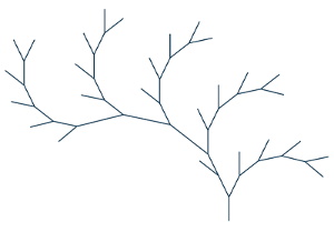
Figure 1 shows the result of a simulation run. The evolved plants use a fan-like growth pattern to spread out the end branches as efficiently as possible, without wasting any structure. The L-system for these plants is surprisingly simple: the axiom is $$A[+B]AAAA$$and the one production rule is$$A \to B[-A]+B$$The system iterates five times to obtain the plant shape in Figure 1. To explore this particular system further, it can be entered in the interactive renderer in my previous blog post on Lindenmayer systems. The simulation software can be found in this GitHub repository, and I've hosted a browser version here. Note that this application uses WebGL 2.0 for rendering.

In summary, evolving Lindenmayer systems with certain properties is very doable. It's time to take further steps to increase the realism of this simulation.

Adding dimensions

Now that the 2D simulation has shown that evolving Lindenmayer systems is viable, a more intricate simulation can be set up. It's not enough to hold the plants to realistic standards; the environment must have some degree of realism as well. The following properties aim to create an environment with realistic properties:

• Both the environment and the plants in it must be three-dimensional.
• Fertility across the environment must vary to simulate natural boundaries, and to enforce diverse plants adapting to different circumstances.
• Competition between plants should be simulated. Plants can compete on different levels, e.g. space, sunlight exposure and reproductive strength.

Making everything three-dimensional is not very hard, since it does not change the process of applying or rendering L-systems. This was mostly an engineering effort. I wrote OpenGL based software in C++ to render these three dimensional simulation environments. The Lindenmayer system interpreter models leaves by filling the space in-between branches after a specific leaf symbol is encountered. The other two goals are a bit more difficult to design.

Environment fertility

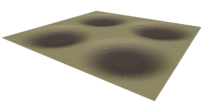
Figure 2 shows an empty simulation environment, representing ground in which plants may grow. Fertility is visualized by making fertile ground darker and lower than infertile areas. In fertile grounds, plants may grow larger (or, in the context of Lindenmayer systems, more iterations of rule application are performed in fertile areas). The amount of material a plant may grow correlates with fertility. The least fertile areas will only support very small plants like grass, while the valleys allow for shrubberies and trees.

The fertility feature has two aims:

• It supports different plant species simultaneously. Small plants on infertile areas will coexist with more complex plants in valleys. This results in a greater genetic diversity within the simulation.
• It creates natural boundaries, causing divergent evolution. At a simpler stage, plants may spread across the entire environment. As time goes on however, they may develop into more complex plants in the valleys, preventing them from escaping their biomes. At this point, two distinct species with a common ancestor have emerged.

Competition

Simulating competition is a threefold issue:

• Plants will compete for sunlight. If sunlight is occluded by the light of other plants, the overshadowed plant will not be successful.
• Plants will compete at the level of reproductive strength. Producing more seeds will increase the chance of one of the seeds sprouting, but this is a tradeoff: producing seeds costs energy.
• Plants will compete for space. They can not grow infinitely dense, if other plants already occupy a certain area, no new plants can sprout there.

Competition for sunlight is implemented through the way leaves work. The fitness of a plant is largely determined by the amount of sunlight its leaves receive in relation to its size. The more sunlight received per mass, the higher the fitness. Leaves are, realistically, not fully opaque. They do however reduce the amount of light that passes through them. If some plants in a simulation evolve taller structures, they will automatically reduce the success of their neighbors by reducing the amount of sunlight they receive. The entire population that experiences occlusion will then favor taller plants.

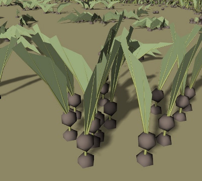
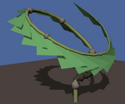
Reproductive strength is modelled through seed production. Figure 3 shows plants with reproductive organs; the brown spheres represent the seeds. When the next generation of plants is produced, a new plant is created for each seed in the environment, not for each plant. The seeds are then ranked by parent plant fitness, after which they sprout in order of fitness score. Plants with a high number of seeds will have a higher chance to reproduce, but creating seeds bears a fitness penalty; plants must therefore evolve to grow an effective number of seeds that is not needlessly high, but at the same time high enough to ensure survival.

Competition for space is implemented by defining a density threshold; the threshold at a certain point in the environment is the number of plant that overlap there. If the number of overlapping plants at a point is over the density threshold, no new plants may sprout there. Combined with the seeds mentioned above, this restriction will only create plants at locations that are not too densely populated. The result of the interplay between seeds and space competition is a new generation that will consist of at least the best plants from the last generation, but also of less successful plants that managed to find an empty spot to grow in.

Results

Simulations were initialized by seeding empty environments with plants consisting of a single seed, and no production rules. This simple plant can only reproduce itself once, without creating any structure apart from the seed. As the simulation progresses and plants reproduce, small mutations give rise to more complex and successful structures by randomly creating and modifying production rules.

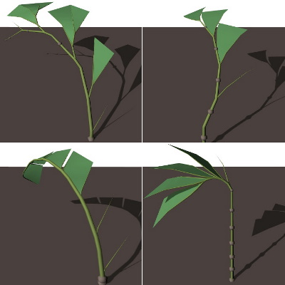
Figure 4 shows four plants obtained from a simulation that ran for about ten thousand generations. These plants share a common ancestor, but they have evolved into different species over time. Their growth patterns are still very similar; leafless branches develop near the base of the plant, and they develop into leaves as the plant grows. The seed growth patterns vary; they grow across the entire plant structure in the top two plants, while they are more concentrated in the others. The leaf placement varies as well. In some plants, they are more spread out, while others try to grow them as high as possible.

These different strategies emerged because the four plants in figure 4 evolved in different valleys (see figure 2); they never grew next to one another. These plants had to compete against different neighbors, requiring different competitive tactics to survive. Some may have competed against plants with lots of seeds, while others had to compete for sunlight.

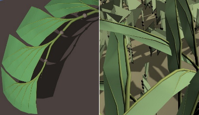
The simulation favors well supported smaller leaf surfaces over large ones, mostly because unsupported surfaces are weak and vulnerable, but also to prevent plants from "cheating" by spanning huge areas with leaf material. Figure 5 shows how plants in the simulation solve this challenge: leaf surfaces are separated by leaf nerves, which are similar and analogous to the way real world leaves structure themselves.

To promote stable structures, the simulation favors plants whose center of gravity is as close to their root as possible. This penalizes both unnecessary tall or skewed structures. This criterion is of course a simplified one. Figure 6 shows a plant that satisfies this constraint very well. Its center of mass is approximately above its root, and it grows quite close to the ground will still exposing all its leaves to the sun. In reality however, this structure would be awkwardly spring-like and unstable. This exposes a limitation in the simplified stability criterion.

The need for competition

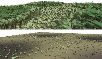
To evaluate the effect of competition on the simulation, two almost equal simulations for 20000 generations were created. The only difference was the density threshold; in one simulation, the density threshold was so low that plants could never really overlap, ruling out competition for sunlight and space. The result was interesting.

Figure 7 shows the end result of the simulations. The one on top had a normal density threshold, while the one on the bottom had a very low one. While more complex plants emerged in the normal simulation, the one without competition had nothing interesting in it. From generation 1500 and onwards, the plants did not change. Their Lindenmayer systems did slowly change through mutation, but they did not add any complexity. This experiment shows that complex plants do not evolve without competition. After all, there is no need to compete without neighbors. A very small plant consisting of nothing more than one leaf (like to the ones in figure 7) is very efficient in this setting.

An interesting property of this competition driven simulation method is that it does not converge, while many commonly used evolutionary algorithms do. Because plants always compete, a stable optimum is never reached. Instead of just competing against a fitness function and settling at some optimum after a while, plants keep competing against each other. The population keeps changing indefinitely.

Conclusion

Evolving Lindenmayer systems as plants definitely yields interesting results. If the fitness function roughly promotes realism, the simulation yields plants that exhibit properties that can be found in nature as well. There are plenty of opportunities to expand on this experiment:

• Flowers can be simulated by increasing the fitness value of plants with "attractive" seeds; the more a seed is surrounded by bright colors, the higher the chance of reproduction becomes.
• Pollinators can be simulated. Plants can fertilize each another, resulting in seeds that contain a Lindenmayer system that is a mix of both parents. The method of combining a genome like this is called crossover.
• Environments can be made more interesting by not just having one-dimensional fertility, but also other factors like nutrition, moisture and temperature. This may result in greater biodiversity.
• Environments can be dynamic by implementing varying climate conditions, or rivers that change over time.
• The Lindenmayer system interpretations can be made more versatile by implementing interpretations for other plant features (fruits, bark, hairs, succulent leaves, needles and so forth). Combined with more complex environments, this could also increase the biodiversity in a simulation.

The source code for this simulation can be found on GitHub, and the in depth paper can be read here.